 Guest
Guest
You need to login to ask any Questions from chapter compressibility-of-soils of soil-mechanics
Chapter:
1. Define consolidation and explain it's types.
The property of soil by virtue of which the volume decreases under applied pressure is termed as compressibility.
The compression of soil can occur due to one or more of the following causes :
Compression of solid particles and water in the voids.
Compression and expulsion of water in the voids.
Expulsion of water in the voids.
The process in which gradual reduction in volume of soil mass occurs under sustained loading and is primarily due to expulsion of pure water is known as consolidation. It is the property of fine grained soil because the fine grained soil mass has large void ratio and higher water content.
The term consolidation applies more to fine grained soil than to coarse grained soil for the following reasons:
Fine grained soil are more compressible than coarse grained soil in therefore the settlement of fine grained soil are generally larger than that of coarse grained soil.
Consolidation of fine grained soil takes much longer time than coarse grained soils due to low permeability. Fine grained soil impose long-term problem to the super-structure.
The consolidation of soil deposit can be divided into three stages:
Initial consolidation
primary consolidation
secondary consolidation
Initial Consolidation:
The reduction in volume of this soil just after the application of the load is known as initial consolidation or initial compression. For saturated soils, the initial consolidation is mainly due to compression of solid particles.
Primary consolidation:
After initial consolidation, further reduction in volume occurs due to expulsion of water from the voids. This reduction in volume is called primary Consolidation which depends upon the permeability of the soil.
In fine grained soils, the primary consolidation occurs over a long time. On the other hand, in course grained soils, the primary consolidation occurs rather quickly due to high permeability.
Secondary Consolidation:
The reduction in volume continues at a very slow rate even after the hydrostatic pressure developed by the applied pressure is fully dissipated and the primary consolidation is complete. This additional reduction in the volume is called secondary consolidation.
2. Explain standard One Dimensional Consolidation Test.
The consolidation test is conducted in a laboratory to study the compressibility of a soil. The test is performed in the consolidation test Apparatus, known as the consolidometer or an oedometer. The following test procedure is applied to any type of soil in the standard consolidation test:
Loads are applied in steps in such a way that the successive load intensity is twice the proceeding on the load intensity is commonly used being `¼`,`½`,`1`,`2`,`4`,`8`, and `16 (kg)/M^2`. Each Load is allowed to stand until compression has practically ceased. The dial readings at elapsed time of `1/ 4`,` ½`, `1`,` 2`,` 4`, `8`, `15`, `30`,`60`,`120`,`240`,` 480` and `1440` minutes from the time the new increment of load is put on the sample. The Sandy samples get compressed in a relative short time as compared to Clay samples.
After the greatest load required for the test has been applied to the soil sample, the load is removed in decrements to provide data for plotting the expansion curve of this soil in order to learn its elastic properties and magnitude of plastic or permanent deformations. The following data should also be obtained:
Moisture content and weight of the soil sample before the commencement of the test.
Moisture content and weight of the sample after the completion of the test.
The specific gravity of the solids.
The temperature of the room where the test is conducted.
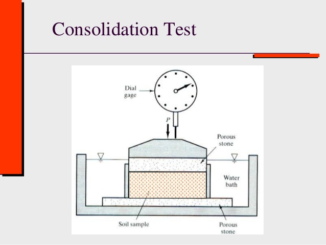
Fig:One dimensional consolidation test
Determination of void ratio:
The results of a consolidation test are plotted in the form of a plot between void ratio and the effective stress. It is therefore, required to determine the boiler ratio at various load increments. There are two methods:
height of solids method
change in void ratio method
The first method is generally applicable to both saturated and unsaturated soils while the second method is applicable only to saturated soil.
Height of solids Method:
In this method,The equivalent height of solid is determined from the dry mass of the soil. The height of solid is given by:
`H_s=V_s/A`
Or,`H_s=W_s/(G*gamma_w)*1/A`........(i)
Where,
`H_s=`Height of solids
`V_s=` volume of solids
`W_s=` dry mass of sample
`G=` specific gravity of solids
`A=` cross sectional area of specimen
We have,
`e=`Volume of voids/Volume of solids
Or,`e=(V-V_s)/V_s`.......(ii)
Now,
`e=((A*H)-(A*H_s))/(A*H_s)`
Or,`e=(H-H_s)/H_s`......(iii)
Where,`H=`final specimen thickness
Thus,
`H=H_0+- sum(triangleH)`
` =H_1+ triangleH`
`H_0=` Initial height of the specimen
`triangleH=` change in the specimen thickness under any pressure increment
`H_1=` height of specimen at the beginning of any load increment
Knowing the void ratio at the beginning and at the end of the test corresponding water content and degree of saturation can be calculated.
Change in Void ratio Method:
Let us assume the specimen to be fully saturated. Now, the void ratio at the end of the test is determined from the following relation:
` e_f=w_f*G`
Where,
`e_f=` final void ratio at the end of the test
`w_f=` final water content at the end of the test
the change of void ratio `triangle e` under each pressure increment is calculated from the following relationship:
`(triangle e)/(1+e)=(triangleH)/H`
Or,`triangle e=(1+e_f)/H_f*triangleH`
Knowing `triangle e` and working backwards from the known value of `e_f`, the equilibrium void ratio corresponding to its pressure can be evaluated.
3. Coefficient of compressibility
Coefficient of compressibility:
The coefficient of compressibility is defined as the decrease in void ratio per unit increase in effective stress. It is equal to the slope of the pressure void curve as shown in the figure.
`a_v=-(triangle e)/(triangle sigma')`......(i)
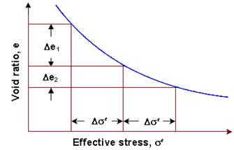
Fig:pressure void ratio curve
The above equation shows that the coefficient of compressibility decreases with increase in effective stress. The above question gives the slope of pressure void curve drawn to a natural scale. This curve has a negative slope which indicate that void ratio decreases as the pressure increases. The slope,`(triangle e)/(triangle sigma')` is called the coefficient of compressibility and is denoted by `a_v`. Thus,in other words the coefficient of compressibility represent the change in void ratio with the change in pressure .
Coefficient of Volume Change:
The coefficient of volume change or volume compressibility is defined as the volumetric strain per unit increase in effective stress.i.e,
`M_v=((triangle V)/V_0)/(triangle sigma)`
Where,
`M_v=`Coefficient of volume change
`V_0=` initial volume
`triangle V=` change in volume
`triangle sigma=` change in effective stress
Let `e_0` be the initial void ratio. let the volume of solid be unity. Therefore, the initial volume `V_0` is equal to `1+e_0`. If `triangle e` is the change in void ratio due to change in volume, we have `triangle V=triangle e`.Thus,
`(triangle V)/(V_0)=(triangle e)/(1+e_0)=`
Thus, the coefficient of volume change is
`m_v=-(triangle e)/(1+e_0)*1/(triangle sigma') `
`Or,m_v=a_v/(1+e_0)`
Compression Index:
The compression index `c_c` is defined as the slope of the linear portion of the void ratio versus `log sigma `plot as shown in the figure .
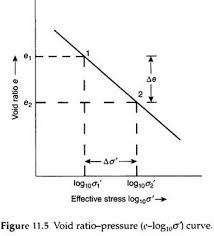
Thus,
`c_c=-(triangle e)/(log_(10)((sigma') /(sigma'_0)) `.....(i)
Where,
`sigma'=`Final effective stress
`sigma_0=`Initial efffective stress
`triangle e=`Change in void ratio
Or, `c_c=- (triangle e)/(log_(10)((sigma'_0+triangle sigma')/(sigma'_0))) `.........(ii)
Where,
`triangle sigma'=`Change in effective stress
The compression index is extremely useful for determination of the settlement in the field. the compression Index of a clay is related to its index properties, especially the liquid limit. Terzaghi and Peck gave the following empirical relationship for clay of low to medium sensitivity
For undisturbed soils,
`c_c=0.009(w_l-10)`
For remolded soils,
`c_c=0.007(w_l-10)`
Expansion Index:
The expansion or swelling index `c_e` is defined as the slope of the void ratio versus `log sigma `plot obtained during unloading (`BEC` in figure).
`c_e=(triangle e)/(log_(10)((sigma'+triangle sigma')/(sigma')))`
Recompression Index:
Recompression is the compression of a soil which had already been loaded and unloaded.The load during the recompression is less than the load to which the soil has been subjected previously. The slope of the recompression curve obtained during reloading (`CFD` in figure) when plotted as the void ratio versus `log sigma ` is equal to the recompression index. Thus,
`c_r=-(triangle e)/(log_(10)((sigma'+triangle sigma')/(sigma')))`

In above figure, the curve AB indicates the decrease in void ratio with an increase in the effective stress.After the sample has reached equilibrium at the effective stress of `sigma_2`, as shown by point B, the pressure is reduced and the sample is allowed to take up water and swell. The curve `BEC` is obtained in unloading. This is known as expansion curve or swelling curve. It may be noted that the soil cannot attain the void ratio existing before the start of the test, and there is always some permanent set or residual deformation.
If the specimen which has swelled to the point C is reloaded, the recompression curve `CFD` is obtained. As the load approaches the maximum value of the load previously applied corresponding to point B, there is reversal of curvature of the curve and then the plot `DG` continues as an extension of the first loading curve `AB`. However, the reloaded specimen remains at a slightly lower void ratio at point `D` than that attained at `B` during the initial compression for the same load.
Normally Consolidated and Over Consolidated Clays:
A clay is said to be normally consolidated if the present effective overburden in pressure is the maximum pressure to which the layer has ever been subjected at any time in its history. That is, if the clay has not been consolidated with stress greater than the present stress, it is called normally consolidated clay.
A clay layer is said to be over-consolidated if the layer was subjected at one time in its history to a greater effective overburden pressure than the present pressure. That is, if the clay has already been subjected to a stress greater than the present stress, it is called overconsolidated clay.
The reasons for over consolidation may be due to following factors:
Weight of an overburden of soil which has eroded.
Construction and unload through the demolition of structure.
Groundwater movement and increase in pore water pressure.
Due to melting of glaciers which covered the soil deposit in the past.
Due to tectonic forces caused by the moment of earths crust.
Due to this desiccation of clay deposit.
The portion `AB` of the above curve represents the soil in normally consolidated condition. The curve in this range is also called the virgin compression curve. The soil in the range CD when it is recompressed represents over-consolidated condition, as the soil had been previously subjected to a pressure `sigma_2`, which is greater than the pressure in the range `CD`.
The maximum pressure to which an overconsolidated soil had been subjected in the past divided by the present pressure is known as overconsolidation ratio (O.C.R).
`OCR=P_c/P_0=(sigma'_c)/(sigma')`
Where,
`P_c (sigma_c)=`maximum effective past pressure
`P_0 (sigma')=`present effective pressure
For normally consolidated clay, `OCR~~1`
For over consolidated clay, `OCR>1`
For example, the soil indicated by the condition at point C as an overconsolidation ratio of `(sigma_2)/(sigma_1)`.
It may be emphasized that normally consolidated soil and overconsolidated soils are not different types of soil but these are the condition in which a soil exists. The same type of soil can behave as a normally consolidated in a certain pressure range and an overconsolidated in some other pressure range. For example, in figure the soil which behaves as overconsolidated In the range `CD` would again behave as normally consolidated in the range `DG`.
The liquidity Index of a normally consolidated clay is generally between 0.6 and 1.00, where is that for Innova consolidated clay is between 0.0 and 0.60.
As the recompression index is very small as compared with the compression index, the soil in the overconsolidated state have smaller compressibility.
If the clay deposit has not reached equilibrium under the applied overburden loads, it is said to be under-consolidated. It is the one which is still to be fully consolidated under the existing overburden pressure. This normally occurs in areas of recent landfills.
4. What is Pre Consolidation Pressure? Explain emperical method for determination of Pre Consolidation Pressure.
Preconsolidation pressure is the mean effective vertical stress that has acted in the clay many times in its history. From pressure void curve, Cassagrande has proposed an empirical method for the estimation of preconsolidation pressure. The procedure is described as below:
Visually determine the point P that has the maximum curvature. Draw a horizontal line PQ. Draw Tangent `PR` at `P`. Draw the line `PS` bisecting the angle `QPR`. Produce the straight line portion of the `e-log(sigma)` plot . Plot backward to intersect `PS` at `T`. The effective pressure corresponding to point `T` is the preconsolidation pressure `sigma_(max)`.
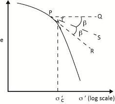
Fig: Graphical procedure for the determination of preconsolidation pressure
5. Explain one dimensional Terzaghi's Theory of Consolidation.
Terzaghi gave the theory for the determination of the rate of consolidation of a saturated soil mass subjected to a static, steady load. The theory is based on the following assumption:
The soil is homogeneous and isotropic.
The soil is fully saturated.
The solid particles and water in the voids are incompressible. The consolidation occurs due to expulsion of water from the voids.
The coefficient of permeability of the soil has the same value at all the points, and it remains constant during the entire period of consolidation.
Darcys law is valid throughout the consolidation process.
Soil is laterally confined, and the consolidation takes place only in axial direction. Drainage of water also occurs only in the vertical direction.
The time lag in consolidation is entirely due to the low permeability of the soil.
There is a unique relationship between the void ratio and effective stress, and this relationship remains constant during the load increment. In other words, the coefficient of compressibility and the coefficient of volume change are constant.
Let us consider a saturated clay layer of thickness 2D sandwiched between two layer of sand is shown in the figure. When a uniform pressure of `triangle sigma` is applied on the surface of the top sand layer ,the total stress developed at all points in the clay layer is increased by `triangle sigma`.
As explained in the spring analogy model, initially the whole of the pressure is taken up by water, and the hydrostatic excess pressure of `(triangle sigma)/gamma_w` develops. At time `t=0`,just after the application of the load, the excess hydrostatic pressure `bar(u_i)` is equal to `(triangle sigma)/gamma_w` throughout the clay layer. This is represented by the original line `AB`. The excess hydrostatic pressure is independent of the position of the water table for convenience, the water table is assumed at the level of the surface of the clay layer.
The hydrostatic excess pressure at the top and the bottom of the clay layer, indicated by point C and D in the pressure diagram drops to zero.However, the excess hydrostatic pressure in the middle portion of the clay layer at `D` remains high. The curve indicating the distribution of excess hydrostatic pressure are known as isochrones. The isochrone `CDE` indicates the distribution of excess hydrostatic pressure at time t.
As the consolidation progress, the excess hydrostatic pressure in the middle of the clay layer decreases. Finally at time `t=t_f`, the whole of the excess hydrostatic pressure has been dissipated, and the pressure distribution is indicated by the horizontal isochrone `CFE`.
Let us consider the equilibrium of an element of the clay at a depth of Z from its top at time t. The consolidation pressure `triangle sigma` is partly carried by water and partly by solid particles as:
`triangle sigma=triangle bar(sigma)+bar(u)`
Where,
`triangle bar(sigma)=`the pressure carried by the solute particles
`bar(u)=`the excess hydrostatic pressure
Now,hydraulic gradient `i` at that depth is,
`i=(delh)/(delz)=(del(bar(u)/gamma_w))/(del z) `
Or,`i=1/gamma_w*(del baru)/(del z)`
Where, `bar u` is the excess hydrostatic pressure at depth `z`.
Let us consider a thin slice of clay layer `triangle z` at depth `z`. Now, the pressure difference across this thickness is given by:
`triangle baru=(bar u+(delbar u)/(del z)*del z)-bar u`
`=(del bar u)/(del z)*dz`
The unbalanced head across the thickness is given by,
`triangle h=(triangle bar u)/gamma_w`
`=1/gamma_w(del bar u)/(del z)*dz`
Thus, the hydraulic gradient becomes,
`i=(triangle h)/dz=1/gamma_w*(del bar u)/(del z)`
Again from darcy law, the velocity of flow at depth `z` is,
`v=k*i=k*1/gamma_w*(del bar u)/(del z)`
The velocity of flow at the bottom of the element of thickness `triangle z` can be written as,
`=v+(del v)/(del z)*dz`
`=v+del/(del z)(k/gamma_w*(del bar u)/(del z))*dz`
Or,`v+(del v)/(delz)dz=v+ k/gamma_w(del^2baru)/(del z^2)*dz`
Or,`(del v)/(del z)=k/gamma_w(del^2baru)/(del z^2)`
The discharge entering the element is,
`Q_(Inp)=v*(trianglex*triangley)`
Where `trianglex` and `triangley` are the dimension of the element.
The discharge leaving the element is,
`Q_(out)=v+(del v)/(del z)*dz(trianglex*triangley)`
Therefore, the net discharge squeezed out of the element is:
`triangle Q=Q_(out)-q_(Inp)`
`=[v+(del v)/(del z)*dz-v](trianglex*triangley)`
`=(del v)/(del z)(trianglex*triangley* triangle z)`
As the water is squeezed out, the effective stress is increased and the volume of the soil mass decreases.
We have,
`triangle V=-m_vV_0 triangle bar(sigma)`
Where,
`V_0=`initial volume of soil mass
`=trianglex*triangley* triangle z`
`triangle bar (sigma)=`Increase in effective stress.
The decrease in volume of soil per unit time is,
`del /(del t)(triangle V)=-m_v*trianglex*triangley* triangle z*del/(del t)(triangle bar sigma)`
As the decrease in volume of soil mass per unit time is equal to the volume of water squeezed out per unit time,We have,
`(del v)/(del z)(trianglex*triangley* triangle z)==-m_v*trianglex*triangley* triangle z*del/(del t)(triangle bar sigma)`
`(del v)/(delz)=-m_v*del/(del t)(triangle bar sigma)`
We know that,
`triangle bar sigma=triangle sigma-bar u`
`del/(delt)(triangle bar sigma)=del/(delt)(triangle sigma)-del/(delt)(bar u)`
For a given pressure increment,`del (triangle sigma)=0`,so,
`del/(delt)(triangle bar sigma)=-del/(delt)(bar u)`
Using this, we get,
`(del v)/(del z)=m_v (del bar u)/(del t)`
Equating the two values of `(delv)/(delz)`, we get,
`k/gamma_w*(del^2bar u)/(del z^2)=m_v*(del bar u)/(del t)`
Or, `c_v*(del^2bar u)/(del z^2)=(del bar u)/(del t)`...........(i)
Where, `c_v=`coefficient of consolidation and is given by,
`c_v=k/(gamma_wm_v)=k/(g rho_w m_v)`
Equation (i) is the basic differential equation of one-dimensional consolidation. It gives the distribution of hydrostatic excess pressure `bar u` with depth `z` and time `t`.
6.
Terzaghi basic differential equation of consolidation can be solved with the following boundary condition:
`z=0`,`u=0`
`z=2d`,`u=0`
`t=0`,`u=u_0`
The solution yields,
`int[2u_0/M sin((Mz)/d)]e^(-M^2T_v)`.........(i) from limit `m=0` to` m=�??`
Where,
`m=` an integer
`M= pi/2*(2m+1)`
`u_0=`initial excess pore water pressure.
`T_v=`Time factor which is non dimensional number
`T_v=(C_v*t)/u_0`
A series of isochrones indicating the variation of `u` and `z` can be plotted for different value of `T_v`. The shape of isochrones depend on `u_0` and drainage condition at the boundary of clay layer.
If both upper and lower boundaries are free draining, the clay layer is known as openlayer. If only one boundary of clay layer is free draining, the layer is called half closed layer.
The progress of consolidation at any point depends upon the pore water pressure `u` at that point. The degree of consolidation at any point `z` is equal to the ratio of the dissipated excess pore water pressure to the initial excess pore water pressure.i.e,
`U_z=(u_0-u_z)/u_0`
`=(1-u_z)/u_0`
Where,`u_z=`excess pore water pressure at time `t`.
The average degree of consolidation for the entire depth of clay layer at any time `t` can be written as:
`U=S_(c(t))/S_c `
$=\int_{0}^{2d} (u_z dz)/u_0$
where, `U=`average degree of consolidation
`S_(c(t))=`settlement of layer at time `t`.
`S_c=`Ultimate settlement of the layer.
Substituting of equation (i) yields,
`U=1-sum 2/M^2*e^(-M^2T_v)`
The variation of `U` and `T_v` is shown in figures:
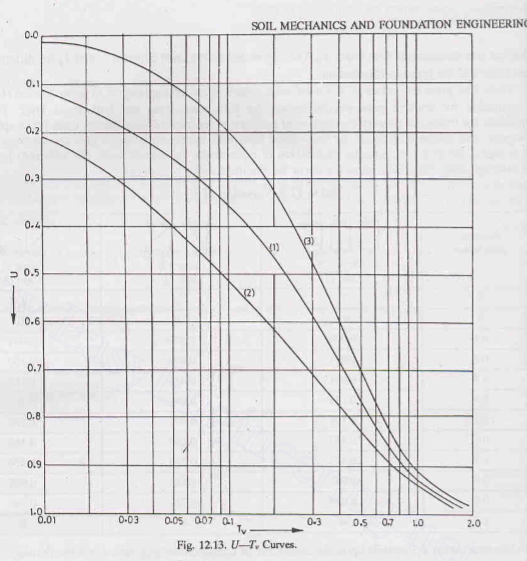
Following plot can be approximated by the expressions given below:
For `U=0` to `60%`,
`T_V=pi/4((U%)/100)^2`
For `U>60%`,
`T_v=1.781-0.933log_(10)(100-U%)`
Or, `T_v=-0.933log_(10)(1-U)-0.085`
Time Factor (`T_v`):
The time factor depends upon the coefficient of consideration (`C_v`) ,time(`t`) and the drainage path `d`.
`T_v=(C_vt)/d^2`
`=(k/(gamma_w m_v))t/d^2 `
`=(k/( m_v*g*rho_w))t/d^2 `
The drainage path `d` represents the maximum distance that the water has to travel before reaching the free drainage boundary.
For Open layer (double drainage),
`d=H/2`
For half closed layer( single drainage),
`d=H`
Where, `H=` thickness of the soil layer
7. Explain Limitation of Consolidation Theory.
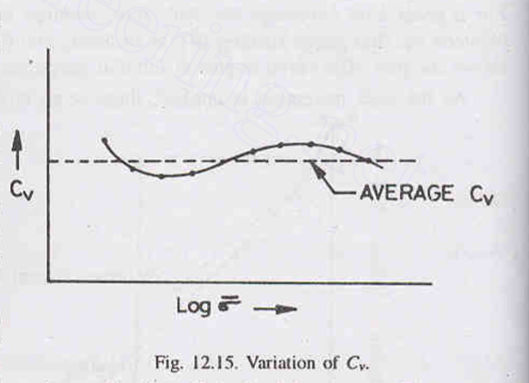
The value of the coefficient of consolidation has been assumed to be constant. However, in reality, it changes with change in the consideration pressur.
The distance `d` of the drainage path cannot be measured accurately in the field.
There is sometimes difficulty in locating the drainage face.
The equation is based on the assumption that the consolidation is one dimensional. In field, the consolidation is generally three-dimensional.
The initial consolidation in the secondary consolidation have been neglected. Sometimes, these form an important part of the total consideration.
In the field, the load is seldom applied instantaneously. The effect of the loading period has to be considered.
In actual practice, the pressure distribution may be far from linear or uniform. The theory become complicated when correct distribution is considered.
8. Explain methods for determinations of Coefficient of Consolidation.
The coefficient of consolidation is determined by methods based on the comparison between the characteristics of the theoretical relation between the time factor, `T_v` and degree of consolidation, `U` to the relation between elapsed time,`t` and degree of consolidation, `U` obtained for soil specimen in laboratory test. Two commonly used methods are:
Logarithm of time fitting method
Square root of time fitting method
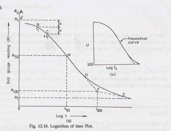
Logarithm of Time Fitting Method:
The method, given by Casagrande, uses the theoretical curve between `U` and `logT_v` as shown as in the figure. The curve consists of three parts:
Initial portion which is parabolic in shape,
a middle portion which is almost linear,
the last portion to which the horizontal axis is an asymptote.
For the given incremental loading of the laboratory test, the specimen deformation against log of time plot is shown in the figure. The following procedures are adopted to determine coefficient of consolidation:
Plot the dial readings for a given load increment against time on semi log graph paper.
Select two points `B` and `C` on the parabolic portion of the consolidation curve which corresponds time `t_1` and `t_2` respectively. Note that `t_2=4t_1` .
Measure the vertical distance between B and C. Say, it is equal to `a` which is at a distance `a` from B.
Set off an equal distance, which is at a distance `a` above the point `B`. Draw a horizontal line, which fixes the point at `R_c`. The dial gauge reading corresponding to this line `R_c` is the corrected zero reading which corresponds to degree of consolidation as zero. The difference between the dial gauge reading at `R_0` and `R_c` is called initial compression.
Project the straight line portion of the two lines `MD` and `DE` to intersect at `F`. The dial gauge reading corresponding to `F` is `R_(100)` i.e, 100% primary consolidation.
Determine the point `M` on the consolidation curve which corresponds to the dial reading`R_(50)` or `(R_c+R_(100))/2`. The time corresponding to the point `M` is `t_(50)` i.e, time for 50% consolidation.
Determine `C_v` from the equation`T_v=(C_v*t)/d^2`. The value of `T_v` for `barU=50%` is `0.197`.Thus, `C_v=0.197d^2/t_(50)`
Square root Time Fitting Method:
This method was developed by Taylor based on the observation of dial gauge reading and time as shown in the figure. The figure shows the form of theoretical and practical curve. The theoretical curve is linear upto about 60% consolidation and at 90% consolidation, the abscissa is `ac=1.15ab`. The practical curve usually consists of a short curve comprising initial portion, a linear part and a second curve.
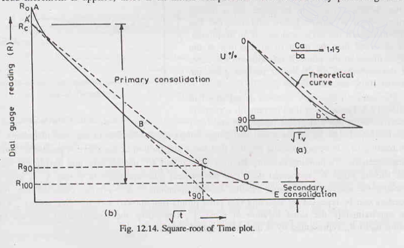
The step by step procedure is given as follows:
plot the dial reading as ordinate with the corresponding is square root of time, `root (2)t` as abscissa.
Produce backward the initial linear part of the curve to intersect at`R_c`. The distance between `R_0` and `R_c` is called initial compression.
Draw a tangent to the line `AB`. Draw the line `AC` such that its abscissa is `1.1 5` times that of the linear portion of `AB`.
The intersection of `AC` with the consolidation curve at `C` will locate `R_(90)` corresponding to `root (2)(t_(90)) ` i.e,the square root of time for 90% of consolidation.
By knowing the`0` and `90%` consolidation, the `100%` consolidation can be obtained.
Beyond `100%` consolidation, it is assumed that the consolidation settlement is completed and secondary consolidation starts.
Find `C_v` by using the equation:`T_v=(C_v*t)/d^2`
The value of `T_v` for `barU=90%` is `0.848`.
So, `C_v=(0.848*d^2)/t_(90)`
9.
The two methods for determination for the coefficient of consolidation give comparable results for most of the soils. However, the following points must be carefully noted:
for some soils, the square root of time plot does not give a straight line for the initial portion and therefore, to locate the corrected zero `R_c` becomes difficult. For such soils, the log of time method is better.
The square root of time method is more suitable for soils exhibiting high secondary consolidation. In such soils, the log t-plot does not show the characteristic shape required to locate the point corresponding to `100%` consolidation.
The square root of time method is more convenient for general case, as it requires dial gauge readings covering a much shorter period of time compared with the log-time method. The latter method requires accurate plotting of the secondary consolidation curve in order to locate the assymptote.